The Travel Problem
Introduction
In this article we will discuss a very common decision problem: how best to travel from a starting point A to some target destination Z in the “best” manner possible. Of course, as we previously discussed in the last article, it is the utility that must be defined in order to quantitatively define what is best. The majority of the article will present the mathematical definition of the utility function $U(x)$ for the travel problem, as well as the reasoning behind the definition, and finally a simple demonstration using simulated flight data.
Utility Function Defined
Before we really get into explaining the reasoning behind our choice of function definition, we will first simply show the mathematical formula in all its glory:
\[U(x) = \frac{D_{\text{ideal}}}{M \cdot T \cdot S \cdot D_{\text{actual}}}\]Where:
- $D_{\text{ideal}}$ is the ideal (straight-line) distance between the start and end points of the journey.
- $D_{\text{actual}}$ is the actual traveled distance.
- $M$ is the monetary cost.
- $T$ is the total time.
- $S$ is the stress.
In the next section we will explore the “reasoning” behind this equation.
Reasoning About Travel Utility
To understand how we arrived at such an equation, we must ask ourselves a simple question: what is the purpose of travel? Simply put, travel is about getting from one point to another. That could be called the “reward” or “benefit.” But the cost of said travel does not include just money $M$, but also time $T$, and even something more abstract, which is stress $S$. So we can think about the “utility” of such a problem as simply:
\[U(x) = \frac{\text{What You Want}}{\text{What It Costs}}\]In this case we want to travel some distance $D$ between two points, but we will be forced to pay some cost term that includes money $M$, time $T$, and stress $S$:
\[U(x) = \frac{D}{M \cdot T \cdot S}\]Distance Efficiency
But there is something else to consider: should utility increase or decrease as we are “forced” to travel more distance than the straight line path?
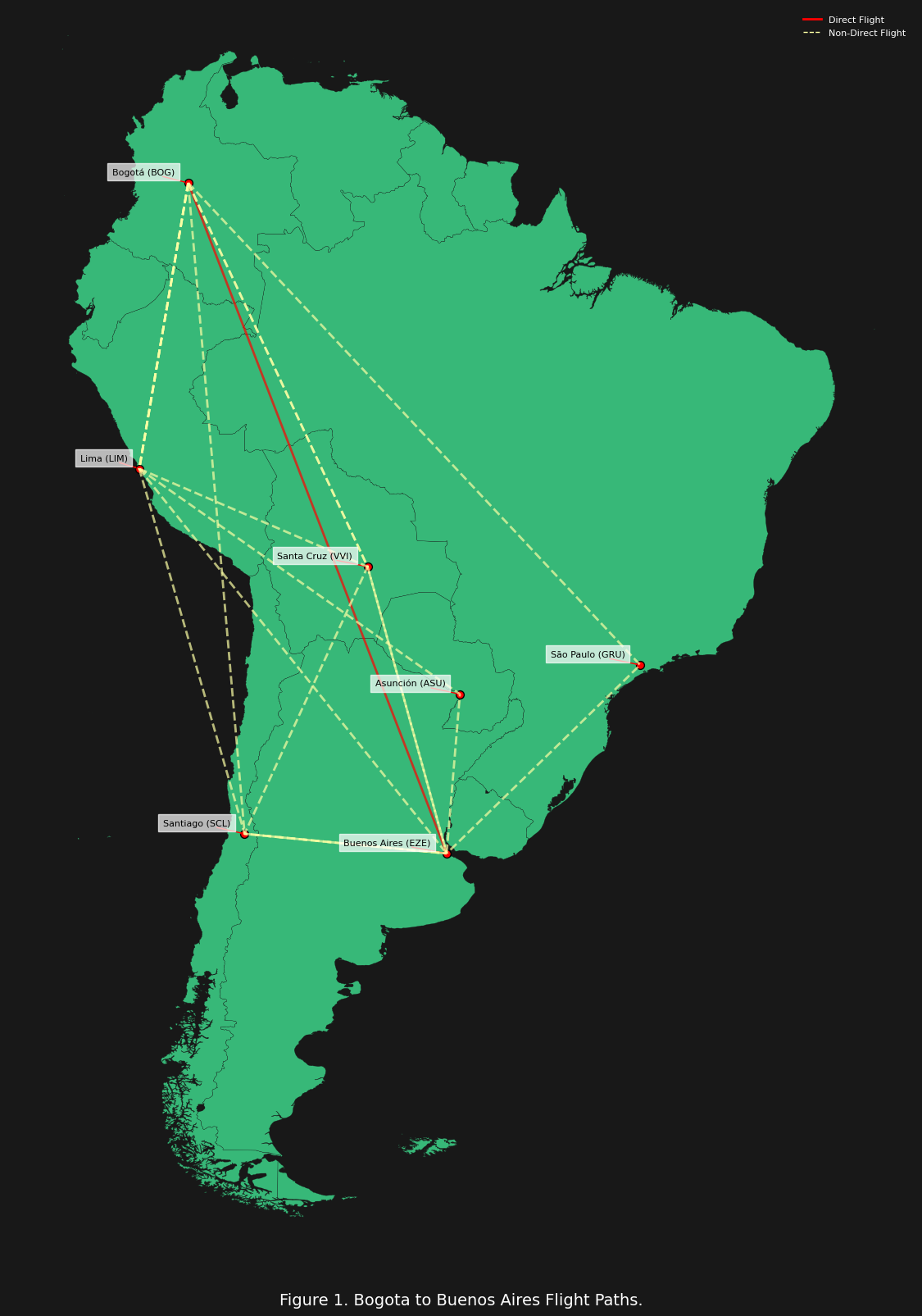
In figure 1 above we can see the various flight paths possible from Bogota, Columbia to Buenos Aires, Argentina. Clearly, any flight path that is not a direct flight will have a longer total distance. Should our utility function reward or penalize this? It would not make sense to “reward” excess distance, because that would be equivalent to “waste” distance. This can be understood in terms of accuracy or efficiency: we do not want to simply travel from point A to Z (e.g. Bogota to Buenos Aires) by any path, we want to get there by the path of minimal waste. So then how do we account for this “waste distance” because clearly we must consider it, otherwise our utility function would be increasing as the distance increases beyond the “ideal distance.” The solution comes from understanding that the “benefit” gained from traveling is not an absolute distance but a distance efficiency ($E_D$):
We are not “buying” raw distance, but instead an “efficiency” or “accuracy” of distance from our origin A to our target destination Z. Now we have the correct behavior:
- $D_{\text{actual}} = D_{\text{ideal}}; E_D = 1$: utility is maximized, since the denominator is just
$M \cdot T \cdot S$, and there is no penalty from the actual distance.
- $D_{\text{actual}} > D_{\text{ideal}}; E_D < 0$: utility decreases as the actual distance grows larger.
We can now simplify the utility function even further:
\[U(x) = \frac{E_D}{M \cdot T \cdot S}\]Mathematics of Stress
The final term of the equation that we need to discuss is stress $S$. The money $M$ and time $T$ terms are relatively simple:
- $M$ represents all the financial costs spent on the trip (e.g. ticket cost, baggage fees, etc …)
- $T$ represents all the temporal costs spent on the trip (e.g. flight time, layovers, traffic, delays, etc …)
But stress $S$ is a bit more abstract and complex:
- Stress accumulates over time, meaning that longer trips generally result in higher total stress.
- Stress grows non-linearly, so a continuous journey without breaks results in disproportionately
more stress than the same duration broken into parts: the whole is more stressful than the sum of its parts.
- Stress growth depends on the traveler’s baseline stress level $S_0$, which represents how sensitive or reactive the traveler is to discomfort, unpredictability, or stimulation.
We “intuitively” feel this: a non-stop, 12-hour flight might feel more stressful than two 6-hour flights with a comfortable layover in between. Conversely, too many layovers can introduce additional stressors such as airport transfers, security checks, and unpredictability.
So how do we go about deriving the mathematical model of stress? Well the “key” insight here is to understand that stress is simply an example of continuously compounding which is just a type of exponential growth:
\[S = S_0 e^{S_0kT}\]where:
- $S_0$ is the baseline stress (initial stress level).
- $k$ is a stress growth rate, which could depend on factors like discomfort, unpredictability, or psychological burden.
- $T$ is the total time spent on that segment of the trip.
Now let us a visualize how this stress equation behaves:
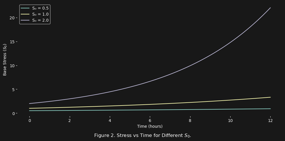
In figure 2 above, what we see is that not only does stress increase with time (in this case flight hours), but the larger $S_0$ (i.e. the higher the base stress) the more exponentially larger the increase in the total stress $S_{\text{total}}$ at the end of the time. We should expect to see the same behavior with the stress growth rate $k$:
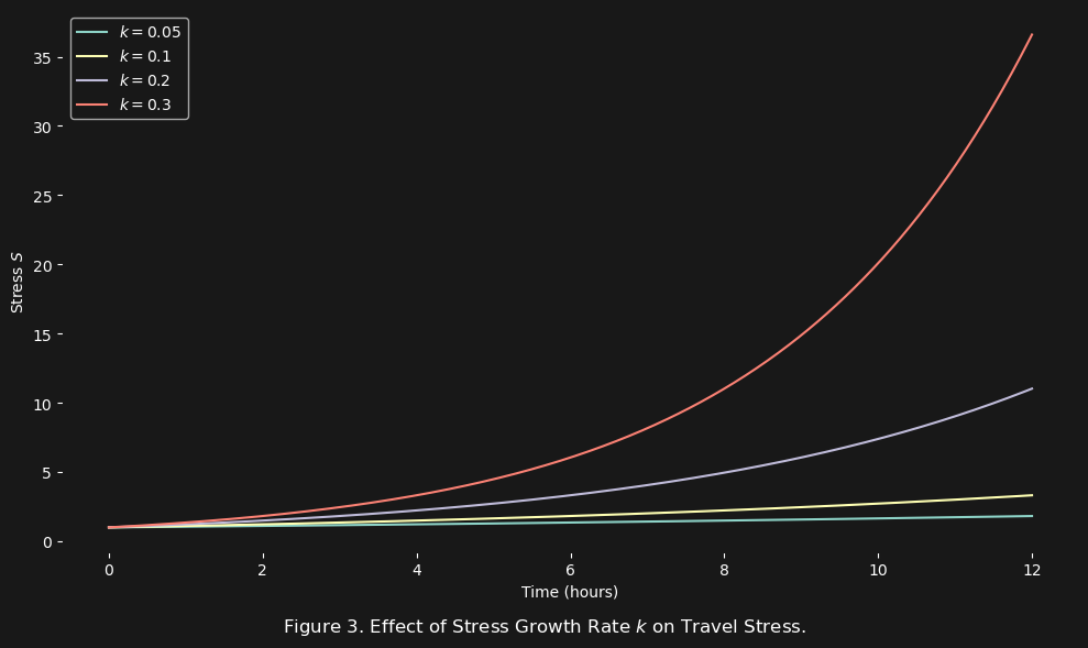
In figure 3 above we see the exact same behavior: the total stress at the end of the travel time period grows exponentially in response to not only time but as we increase the growth rate $k$. Basically, any term that should influence the growth rate of stress $S$ should be in the exponent of the stress growth equation. Hence why both $S_0$, $k$, and $T$ are in the exponent:
\[S = S_0 e^{S_0kT}\]And what is so special about the exponent that it influences the growth rate? The derivative:
\[\frac{dS}{dt} = \frac{d}{dt} \left( S_0 e^{S_0 k t} \right) = S_0^2 k e^{S_0 k t}\]Whatever is in the exponent of the equation will be in the exponent of its derivative (exponentially influencing the stress growth rate) and that is exactly where we want $S_0$, $k$, and $T$ to be.
Finally, we want there to be a difference between continuous and interrupted stress:
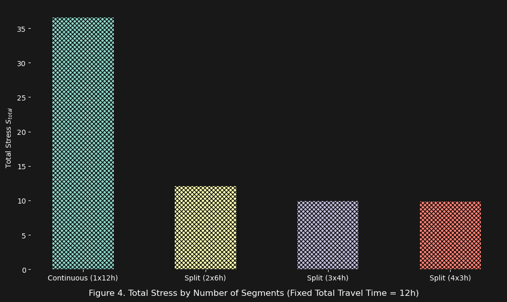
In figure 4 above we see the results of the same flight trip broken up into different segments:
- $1$ 12-hour segment
- $2$ 6-hour segments
- $3$ 4-hour segments
- $4$ 3-hour segments
And the results are exactly what we want to model in our stress equation: the cumulative stress exponentially decreases.
Synthetic Travel Data
With the stress mathematics defined, we are ready to actually apply the travel utility function to the previous travel plan (i.e. Bogota -> Buenos Aires). But we first will need to generate some synthetic travel data that allows us to simulate what the travel options might look like:
                         Route    Airline    Class  Day Month Time of Day Weather  D_actual
id
499              Direct Flight   Jetsmart  Economy  Sun   Aug     Red-Eye  Cloudy   4670.52
258             Via Santa Cruz       Azul  Economy  Sun   May     Red-Eye   Windy   4701.96
399                   Via Lima   Viva Air  Economy  Thu   Nov     Red-Eye   Clear   5029.47
805               Via Santiago   Viva Air  Economy  Mon   Jun     Red-Eye   Clear   5395.47
874              Via São Paulo   Jetsmart  Economy  Sat   Jan     Morning   Clear   6002.64
52       Via Lima & Santa Cruz        Gol  Economy  Fri   Sep     Red-Eye  Cloudy   5441.00
423        Via Lima & Santiago  Amaszonas  Economy  Thu   Apr     Evening   Clear   5496.03
267        Via Lima & Asunción   Jetsmart  Economy  Thu   Sep     Evening  Cloudy   5450.82
527  Via Santa Cruz & Santiago        Gol  Economy  Sat   Jan     Red-Eye   Rainy   5803.52


     T_flight  T_layover    M ($)         Lounges  S_0  S_flight  S_layover  S_total      U_t
id
499      6.23       0.00   595.49            None  low      6.48       0.00     6.48  4163.59
258      6.27       4.83   775.82            None  low      5.20       1.83     7.02  1641.56
399      6.71       3.95   784.60         Premium  low      5.64       1.47     7.11  1562.60
805      7.19       4.42   712.20           Basic  low      7.41       1.82     9.23  1134.11
874      8.00       2.28   765.34            None  low      8.59       1.44    10.03   985.63
52       7.25       4.19   938.57  Premium + None  low      6.36       2.60     8.96   891.57
423      7.33       4.56   865.63     None + None  low      6.47       2.82     9.29   888.92
267      7.27       4.56  1007.72   VIP + Premium  low      6.82       2.46     9.27   775.06
527      7.74       4.36  1131.69      VIP + None  low      6.84       2.47     9.31   631.24
Here is a breakdown of what each column in the above sample data represents:
Route: The specific flight route taken, including possible layovers or connections.Airline: The airline or airlines providing the travel service. If multiple airlines are used, they are separated by a+symbol.Class: The travel class for the majority of the trip, which influences stress and comfort (e.g., Economy, Business, First Class).Day: The day of the week on which the journey begins (e.g., Mon, Tue, Wed).Month: The month in which the journey begins (e.g., Jan, Feb, Mar).Time of Day: The approximate time of day when the flight begins (e.g., Morning, Afternoon, Evening, Red-Eye).Weather: Weather conditions during takeoff or landing, which can influence stress (e.g., Clear, Cloudy, Stormy, Windy).D_actual: The actual distance covered by the route in miles, which may be greater than the ideal distance due to layovers or deviations.T_flight: Total inflight time in hours.T_layover: Total layover time in hours.M ($): Total monetary cost of the journey in U.S. dollars.Lounges: Available lounges or relaxation areas during layovers, which affect stress (e.g., VIP, Basic, Premium, Private Room).S_0: Initial stress level, which starts at a moderate value for all options but can escalate based on various factors.S_flight: Stress accumulated during the flight, influenced by factors such as class, flight duration, and weather.S_layover: Stress accumulated during layovers, influenced by factors such as available lounges, duration, and crowd density.S_total: Total stress for the entire journey, calculated as the sum ofS_flightandS_layover.U_t: The calculated travel utility score for the route, where higher values represent better travel options.
The $U_t$ column is calculated using the travel utility function:
\[U_t = \frac{D_\text{ideal}}{M \times (T_\text{flight} + T_\text{layover}) \times S_\text{total} \times D_\text{actual}}\]Higher utility values indicate more favorable travel options considering distance, cost, stress, and time. The $D_{\text{actual}}$ values vary depending on different stopovers and connecting routes, which can increase total distance traveled.
Base Stress ($S_0$) Effects
Now that we have a way of generating synthetic flight data, we can explore how different base stress $S_0$ affects the travel utility $U_t$ of the different flight routes. For these comparisons, we will set all the flight parameters to constant values, and simply change the $S_0$ value from low, to moderate, to high.

In figure 5 above we can see that with $S_0$ being set to low stress (i.e. $S_0 = 1$) the highest travel utility flight route is the direct flight straight from BOG to EZE. The question is of course why?
                        Route  Airline    Class  Day Month Time of Day Weather  D_actual
id
0               Direct Flight  Avianca  Economy  Sun   Apr     Red-Eye   Clear   4670.52
4              Via Santa Cruz  Avianca  Economy  Sun   Apr     Red-Eye   Clear   4701.96
2                    Via Lima  Avianca  Economy  Sun   Apr     Red-Eye   Clear   5029.47
3                Via Santiago  Avianca  Economy  Sun   Apr     Red-Eye   Clear   5395.47
1               Via São Paulo  Avianca  Economy  Sun   Apr     Red-Eye   Clear   6002.64
7       Via Lima & Santa Cruz  Avianca  Economy  Sun   Apr     Red-Eye   Clear   5441.00
6         Via Lima & Asunción  Avianca  Economy  Sun   Apr     Red-Eye   Clear   5450.82
5         Via Lima & Santiago  Avianca  Economy  Sun   Apr     Red-Eye   Clear   5496.03
8   Via Santa Cruz & Santiago  Avianca  Economy  Sun   Apr     Red-Eye   Clear   5803.52


    T_flight  T_layover   M ($)      Lounges  S_0  S_flight  S_layover  S_total      U_t
id
0       6.23          0  770.64         None  low      5.05       0.00     5.05  4127.38
4       6.27          3  775.82         None  low      4.57       1.45     6.02  2293.79
2       6.71          3  829.86         None  low      4.89       1.45     6.35  1815.86
3       7.19          3  890.25         None  low      5.86       1.45     7.31  1304.01
1       8.00          3  990.44         None  low      6.27       1.45     7.73   924.18
7       7.25          6  897.77  None + None  low      5.63       2.91     8.54   844.48
6       7.27          6  899.39  None + None  low      5.76       2.91     8.66   828.69
5       7.33          6  906.85  None + None  low      5.76       2.91     8.67   810.78
8       7.74          6  957.58  None + None  low      6.03       2.91     8.94   684.59
Looking at the above travel utility data for figure 5 we see that the direct flight has the lowest $D_{\text{actual}}$ (which means the distance efficiency $E_D$ is the highest), the lowest total stress $S_{\text{total}}$ (because of the lack of layovers), and the lowest cost $M$. So basically when the base stress $S_0$ is low, then the travel utility $U_t$ is dominated by the distance, the layovers and the price.
Now let us consider the scenario where base stress $S_0$ is moderate (i.e. $S_0 = 5$).

In figure 6 above, now that the base stress is set to moderate, we see the direct flight no longer has the highest travel utility.
                        Route  Airline    Class  Day Month Time of Day Weather  D_actual
id
4              Via Santa Cruz  Avianca  Economy  Sun   Apr     Red-Eye   Clear   4701.96
7       Via Lima & Santa Cruz  Avianca  Economy  Sun   Apr     Red-Eye   Clear   5441.00
5         Via Lima & Santiago  Avianca  Economy  Sun   Apr     Red-Eye   Clear   5496.03
6         Via Lima & Asunción  Avianca  Economy  Sun   Apr     Red-Eye   Clear   5450.82
2                    Via Lima  Avianca  Economy  Sun   Apr     Red-Eye   Clear   5029.47
8   Via Santa Cruz & Santiago  Avianca  Economy  Sun   Apr     Red-Eye   Clear   5803.52
0               Direct Flight  Avianca  Economy  Sun   Apr     Red-Eye   Clear   4670.52
3                Via Santiago  Avianca  Economy  Sun   Apr     Red-Eye   Clear   5395.47
1               Via São Paulo  Avianca  Economy  Sun   Apr     Red-Eye   Clear   6002.64


    T_flight  T_layover   M ($)      Lounges       S_0  S_flight  S_layover   S_total    U_t
id
4       6.27          3  775.82         None  moderate    752.88      32.60    785.48  17.58
7       7.25          6  897.77  None + None  moderate    357.33      65.21    422.54  17.07
5       7.33          6  906.85  None + None  moderate    528.49      65.21    593.70  11.84
6       7.27          6  899.39  None + None  moderate    555.82      65.21    621.03  11.56
2       6.71          3  829.86         None  moderate   1282.93      32.60   1315.53   8.76
8       7.74          6  957.58  None + None  moderate    780.32      65.21    845.52   7.24
0       6.23          0  770.64         None  moderate  16399.51       0.00  16399.51   1.27
3       7.19          3  890.25         None  moderate   8064.63      32.60   8097.23   1.18
1       8.00          3  990.44         None  moderate   9144.64      32.60   9177.24   0.78
We can see immediately that the direct flight has the highest $S_{\text{total}}$ value, and the lowest $S_{\text{layover}}$, though still maintaining the highest $E_D$ value. Also notice that there are flights that have a higher $T_{\text{flight}}$, but have a higher $U_t$ value. Why is that? Because those flights have less continuous flight time, which is exactly why their $S_{\text{total}}$ is lower than the direct flight.
This fits the intuition about stress $S$ when it comes to travel: the sum of the whole is greater than the sum of the parts. The stress is not the same for a trip of 6 hours continuous travel, versus a trip of 3 hours travel, 3 hours break, 3 hours travel etc … and this is exactly what we expect to see when modeling $S$ related to travel.
Finally let us take a look at high stress travelers (i.e. $S_0 = 8$).

Finally in figure 7 with the base stress set to high, we have complete dominance of the stress term $S$, and multiple layovers are valued at a higher travel utility $U_t$, simply because they reduce the $S_{\text{flight}}$.
                        Route  Airline    Class  Day Month Time of Day Weather  D_actual
id
7       Via Lima & Santa Cruz  Avianca  Economy  Sun   Apr     Red-Eye   Clear   5441.00
5         Via Lima & Santiago  Avianca  Economy  Sun   Apr     Red-Eye   Clear   5496.03
4              Via Santa Cruz  Avianca  Economy  Sun   Apr     Red-Eye   Clear   4701.96
6         Via Lima & Asunción  Avianca  Economy  Sun   Apr     Red-Eye   Clear   5450.82
8   Via Santa Cruz & Santiago  Avianca  Economy  Sun   Apr     Red-Eye   Clear   5803.52
2                    Via Lima  Avianca  Economy  Sun   Apr     Red-Eye   Clear   5029.47
3                Via Santiago  Avianca  Economy  Sun   Apr     Red-Eye   Clear   5395.47
0               Direct Flight  Avianca  Economy  Sun   Apr     Red-Eye   Clear   4670.52
1               Via São Paulo  Avianca  Economy  Sun   Apr     Red-Eye   Clear   6002.64


    T_flight  T_layover   M ($)      Lounges   S_0    S_flight  S_layover     S_total     U_t
id
7       7.25          6  897.77  None + None  high     3920.51     321.37     4241.88  170.06
5       7.33          6  906.85  None + None  high     9196.52     321.37     9517.89   73.87
4       6.27          3  775.82         None  high    19169.53     160.68    19330.22   71.46
6       7.27          6  899.39  None + None  high    10275.07     321.37    10596.44   67.76
8       7.74          6  957.58  None + None  high    19199.02     321.37    19520.39   31.34
2       6.71          3  829.86         None  high    49595.41     160.68    49756.09   23.17
3       7.19          3  890.25         None  high  1077084.60     160.68  1077245.28    0.89
0       6.23          0  770.64         None  high  3376503.36       0.00  3376503.36    0.62
1       8.00          3  990.44         None  high  1305931.19     160.68  1306091.87    0.55
We can now see from figure 7 and the utility data above that routes with the highest continuous flight times are ranked at the bottom (i.e. Via Santiago, Direct Flight, and Via São Paulo). Whereas flight routes with the lowest $D_{\text{actual}}$, and the lowest continuous flight times (which lowers $S_{\text{flight}}$) are competing at the top (i.e. Via Lima & Santa Cruz, Via Lima & Santiago, and Via Santa Cruz).
Stress Growth Rate ($k$) effects
We have seen the significant influence that the base stress $S_0$ can produce on the travel utility $U_t$. Now we will focus on purely considering how the stress growth rate $k$ can affect $U_t$. We will consider basically the highest and lowest $k$ possible (i.e. the worst and best possible conditions) for travelers of different base stress $S_0$.
First we will consider the worst case scenario for our low stress traveler.

What figure 8 above shows us, is that with a sufficiently high $k$ the travel utility of reducing the continuous flight time begins to increase. We can see this in the corresponding data.
                        Route   Airline    Class  Day Month Time of Day Weather  D_actual
id
0               Direct Flight  Jetsmart  Economy  Fri   Jul     Morning  Stormy   4670.52
4              Via Santa Cruz  Jetsmart  Economy  Fri   Jul     Morning  Stormy   4701.96
2                    Via Lima  Jetsmart  Economy  Fri   Jul     Morning  Stormy   5029.47
3                Via Santiago  Jetsmart  Economy  Fri   Jul     Morning  Stormy   5395.47
7       Via Lima & Santa Cruz  Jetsmart  Economy  Fri   Jul     Morning  Stormy   5441.00
6         Via Lima & Asunción  Jetsmart  Economy  Fri   Jul     Morning  Stormy   5450.82
5         Via Lima & Santiago  Jetsmart  Economy  Fri   Jul     Morning  Stormy   5496.03
1               Via São Paulo  Jetsmart  Economy  Fri   Jul     Morning  Stormy   6002.64
8   Via Santa Cruz & Santiago  Jetsmart  Economy  Fri   Jul     Morning  Stormy   5803.52


    T_flight  T_layover   M ($)      Lounges  S_0  S_flight  S_layover  S_total      U_t
id
0       6.23          0  595.49         None  low     11.34       0.00    11.34  2377.18
4       6.27          3  599.50         None  low      6.96       1.77     8.72  2049.06
2       6.71          3  641.26         None  low      7.79       1.77     9.55  1561.60
3       7.19          3  687.92         None  low     10.96       1.77    12.73   969.64
7       7.25          6  693.73  None + None  low      7.72       3.54    11.26   829.07
6       7.27          6  694.98  None + None  low      8.10       3.54    11.63   798.84
5       7.33          6  700.74  None + None  low      8.09       3.54    11.62   782.75
1       8.00          3  765.34         None  low     11.88       1.77    13.65   676.91
8       7.74          6  739.95  None + None  low      8.71       3.54    12.25   646.35
We can see that, while the ranking of the routes remains mostly unchanged compared to figure 5 (except that the Via São Paulo route dropped quite a bit), the difference in $U_t$ of the top two ranked routes is now smaller (about 300 utility units vs. about 2000 utility units previously). What this suggests, is that even for the low stress traveler, at least one layover (e.g. the Via Santa Cruz route) becomes a far more favorable option when the conditions are significantly unfavorable.
Now let us consider the best case scenario (i.e. low $k$) for our high stress traveler.

The results of figure 9 for the high $S_0$ and low $k$ indicate that for the high stress traveler, not much changes about the ranking of the flight routes even with the most favorable k possible.
                        Route   Airline        Class  Day Month Time of Day Weather  D_actual
id
7       Via Lima & Santa Cruz  Viva Air  First Class  Sun   Oct     Red-Eye   Clear   5441.00
5         Via Lima & Santiago  Viva Air  First Class  Sun   Oct     Red-Eye   Clear   5496.03
4              Via Santa Cruz  Viva Air  First Class  Sun   Oct     Red-Eye   Clear   4701.96
6         Via Lima & Asunción  Viva Air  First Class  Sun   Oct     Red-Eye   Clear   5450.82
8   Via Santa Cruz & Santiago  Viva Air  First Class  Sun   Oct     Red-Eye   Clear   5803.52
2                    Via Lima  Viva Air  First Class  Sun   Oct     Red-Eye   Clear   5029.47
0               Direct Flight  Viva Air  First Class  Sun   Oct     Red-Eye   Clear   4670.52
3                Via Santiago  Viva Air  First Class  Sun   Oct     Red-Eye   Clear   5395.47
1               Via São Paulo  Viva Air  First Class  Sun   Oct     Red-Eye   Clear   6002.64


    T_flight  T_layover    M ($)                      Lounges   S_0    S_flight  S_layover     S_total    U_t
id
7       7.25          6  5223.36  Private Room + Private Room  high     3215.76      29.15     3244.91  38.21
5       7.33          6  5276.19  Private Room + Private Room  high     7164.59      29.15     7193.75  16.80
4       6.27          3  4513.89                 Private Room  high    14379.63      14.58    14394.21  16.49
6       7.27          6  5232.79  Private Room + Private Room  high     7954.35      29.15     7983.50  15.46
8       7.74          6  5571.38  Private Room + Private Room  high    14421.79      29.15    14450.95   7.28
2       6.71          3  4828.29                 Private Room  high    35644.23      14.58    35658.81   5.56
0       6.23          0  2241.85                         None  high  2051665.35       0.00  2051665.35   0.35
3       7.19          3  5179.65                 Private Room  high   683922.95      14.58   683937.53   0.24
1       8.00          3  5762.53                 Private Room  high   823242.93      14.58   823257.51   0.15
The corresponding data for figure 9 corroborates this same conclusion. Interestingly the Direct Flight route actually becomes more favorable with lower $k$ compared to the data for figure 7. At first glance this might seem odd, but on closer inspection we can see that the lower $k$ value means that the Direct Flight is more tolerable, but the increased distance and cost ($M$) of the Via Santiago and Via São Paulo routes is now less tolerable. A subtle but crucial scenario is illustrated by this data: sometimes a litte bit more stress is better than a much longer and more expensive trip.
Also we can see that the actual $U_t$ values are lower for the data used in figure 9 vs. figure 7, and this is due to the significantly higher $M$ value (i.e. cost) that is required for some of these more “premium” options (better airline, ticket class, and layover experience).
And finally let us look at moderate stress travelers, and how they handle the best and worst scenarios, staring with the best scenario (i.e. low $k$).
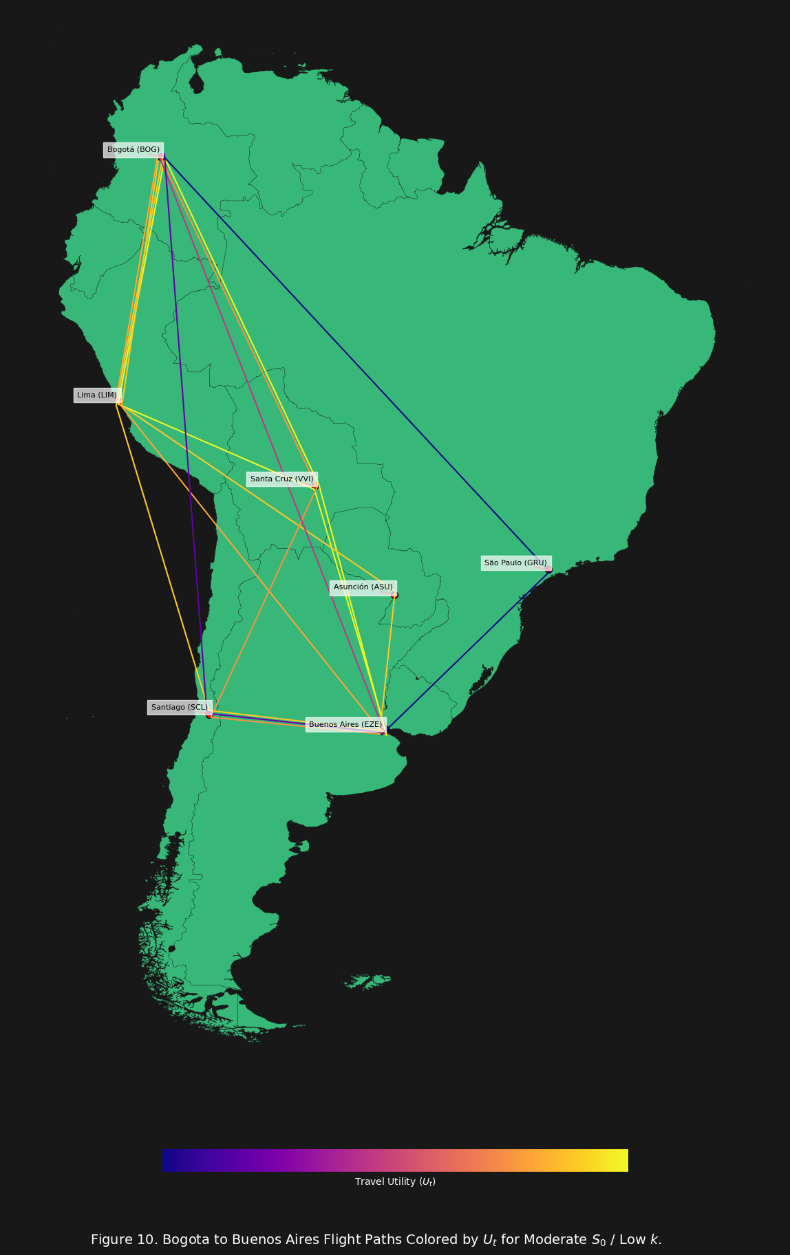
Not much actually changes in this scenario for the moderate stress traveler with a low $k$ (shown in figure 10. In fact it is relatively similar to what we see in figure 6. The only change is simply the higher cost ($M$) reduces the $U_t$ value for all routes.
                        Route   Airline        Class  Day Month Time of Day Weather  D_actual
id
7       Via Lima & Santa Cruz  Viva Air  First Class  Sun   Oct     Red-Eye   Clear   5441.00
4              Via Santa Cruz  Viva Air  First Class  Sun   Oct     Red-Eye   Clear   4701.96
5         Via Lima & Santiago  Viva Air  First Class  Sun   Oct     Red-Eye   Clear   5496.03
6         Via Lima & Asunción  Viva Air  First Class  Sun   Oct     Red-Eye   Clear   5450.82
2                    Via Lima  Viva Air  First Class  Sun   Oct     Red-Eye   Clear   5029.47
8   Via Santa Cruz & Santiago  Viva Air  First Class  Sun   Oct     Red-Eye   Clear   5803.52
0               Direct Flight  Viva Air  First Class  Sun   Oct     Red-Eye   Clear   4670.52
3                Via Santiago  Viva Air  First Class  Sun   Oct     Red-Eye   Clear   5395.47
1               Via São Paulo  Viva Air  First Class  Sun   Oct     Red-Eye   Clear   6002.64


    T_flight  T_layover    M ($)                      Lounges       S_0  S_flight  S_layover   S_total   U_t
id
7       7.25          6  5223.36  Private Room + Private Room  moderate    316.01      14.55    330.56  3.75
4       6.27          3  4513.89                 Private Room  moderate    632.63       7.27    639.90  3.71
5       7.33          6  5276.19  Private Room + Private Room  moderate    455.57      14.55    470.12  2.57
6       7.27          6  5232.79  Private Room + Private Room  moderate    477.39      14.55    491.94  2.51
2       6.71          3  4828.29                 Private Room  moderate   1050.12       7.27   1057.40  1.87
8       7.74          6  5571.38  Private Room + Private Room  moderate    658.74      14.55    673.29  1.56
0       6.23          0  2241.85                         None  moderate  12011.72       0.00  12011.72  0.60
3       7.19          3  5179.65                 Private Room  moderate   6077.65       7.27   6084.93  0.27
1       8.00          3  5762.53                 Private Room  moderate   6865.96       7.27   6873.24  0.18
But what about for moderate stress and high $k$?

What actually seems to happen to moderate stress travelers who are traveling in a high $k$ scenario, is that the relative route rankings begins to look like what we see in high stress travelers (shown in figure 7).
                        Route   Airline    Class  Day Month Time of Day Weather  D_actual
id
7       Via Lima & Santa Cruz  Jetsmart  Economy  Fri   Jul     Morning  Stormy   5441.00
4              Via Santa Cruz  Jetsmart  Economy  Fri   Jul     Morning  Stormy   4701.96
5         Via Lima & Santiago  Jetsmart  Economy  Fri   Jul     Morning  Stormy   5496.03
6         Via Lima & Asunción  Jetsmart  Economy  Fri   Jul     Morning  Stormy   5450.82
8   Via Santa Cruz & Santiago  Jetsmart  Economy  Fri   Jul     Morning  Stormy   5803.52
2                    Via Lima  Jetsmart  Economy  Fri   Jul     Morning  Stormy   5029.47
3                Via Santiago  Jetsmart  Economy  Fri   Jul     Morning  Stormy   5395.47
0               Direct Flight  Jetsmart  Economy  Fri   Jul     Morning  Stormy   4670.52
1               Via São Paulo  Jetsmart  Economy  Fri   Jul     Morning  Stormy   6002.64


    T_flight  T_layover   M ($)      Lounges       S_0   S_flight  S_layover    S_total     U_t
id
7       7.25          6  693.73  None + None  moderate    1775.86     172.88    1948.74  479.04
4       6.27          3  599.50         None  moderate    7511.74      86.44    7598.18  235.26
5       7.33          6  700.74  None + None  moderate    3832.69     172.88    4005.57  227.16
6       7.27          6  694.98  None + None  moderate    4238.38     172.88    4411.25  210.65
8       7.74          6  739.95  None + None  moderate    7541.48     172.88    7714.36  102.62
2       6.71          3  641.26         None  moderate   18127.62      86.44   18214.05   81.92
3       7.19          3  687.92         None  moderate  321822.40      86.44  321908.84    3.83
0       6.23          0  595.49         None  moderate  939206.58       0.00  939206.58    2.87
1       8.00          3  765.34         None  moderate  385635.78      86.44  385722.22    2.40
This makes sense when we consider the structure of the stress equation:
\[S = S_0 e^{S_0kT}\]The exponent term can either be increased by $S_0$, $k$, or $T$. So even if $S_0$ is low, we can still increase the growth rate to a point where it is comparable to a high stress individual. To put it a bit more mathematically:
\[\begin{aligned} S_0 e^{S_0kT} \\ S_0 e^{5\cdot8\cdot1} \\ S_0 e^{8\cdot5\cdot1} \end{aligned}\]In other words a high stress individual (with $S_0 = 8$, $k = 5$, and $T =1$) will have the same stress as a moderate stress individual (with $S_0 = 5$, $k = 8$, and $T = 1$).
Layover ($T_{\text{layover}}$) Effects
The final section we will be discussing involves looking at how the layover times (i.e. $T_{\text{layover}}$) affect the $U_t$ and the relative route rankings. In our discussion we will be asking this key question: is there a point where the layovers are too long that they are no longer an advantage and are now simply a cost? Previously we have seen that as the total stress $S_{\text{flight}}$ increases, there is more preference for layovers. Of course this is because they only interrupt the continuous flight stress. But what happens as those layover times increase?
Let us focus our attention on the high stress traveler, since they are the ones who benefit most from the layovers. First we will consider the 3 hour layover scenario, with the highest $k$ (which will serve more as a baseline).

So as we would expect, the highest ranked routes still have layovers.
                        Route   Airline    Class  Day Month Time of Day Weather  D_actual
id
7       Via Lima & Santa Cruz  Jetsmart  Economy  Fri   Jul     Morning  Stormy   5441.00
5         Via Lima & Santiago  Jetsmart  Economy  Fri   Jul     Morning  Stormy   5496.03
6         Via Lima & Asunción  Jetsmart  Economy  Fri   Jul     Morning  Stormy   5450.82
4              Via Santa Cruz  Jetsmart  Economy  Fri   Jul     Morning  Stormy   4701.96
8   Via Santa Cruz & Santiago  Jetsmart  Economy  Fri   Jul     Morning  Stormy   5803.52
2                    Via Lima  Jetsmart  Economy  Fri   Jul     Morning  Stormy   5029.47
3                Via Santiago  Jetsmart  Economy  Fri   Jul     Morning  Stormy   5395.47
1               Via São Paulo  Jetsmart  Economy  Fri   Jul     Morning  Stormy   6002.64
0               Direct Flight  Jetsmart  Economy  Fri   Jul     Morning  Stormy   4670.52


    T_flight  T_layover   M ($)      Lounges   S_0      S_flight  S_layover       S_total      U_t
id
7       7.25          6  693.73  None + None  high  5.218151e+04    1529.34  5.371084e+04  1738.07
5       7.33          6  700.74  None + None  high  2.509909e+05    1529.34  2.525203e+05   360.32
6       7.27          6  694.98  None + None  high  3.040769e+05    1529.34  3.056062e+05   304.07
4       6.27          3  599.50         None  high  8.418206e+05     764.67  8.425853e+05   212.15
8       7.74          6  739.95  None + None  high  8.393724e+05    1529.34  8.409017e+05    94.15
2       6.71          3  641.26         None  high  3.747737e+06     764.67  3.748501e+06    39.80
3       7.19          3  687.92         None  high  3.951095e+08     764.67  3.951102e+08     0.31
1       8.00          3  765.34         None  high  5.271413e+08     764.67  5.271421e+08     0.18
0       6.23          0  595.49         None  high  2.193592e+09       0.00  2.193592e+09     0.12
The corresponding data for figure 12 above corroborates this conclusion: 3 hour layovers are short enough to contribute less total stress than continous flights. Hence the routes with the most layovers dominates the route rankings in this scenario.
Now let us increase the layover time to 6 hours and see what changes.

There still does not seem to be a lot of change. Let us look at the corresponding data and see what is happening.
                        Route   Airline    Class  Day Month Time of Day Weather  D_actual
id
7       Via Lima & Santa Cruz  Jetsmart  Economy  Fri   Jul     Morning  Stormy   5441.00
5         Via Lima & Santiago  Jetsmart  Economy  Fri   Jul     Morning  Stormy   5496.03
4              Via Santa Cruz  Jetsmart  Economy  Fri   Jul     Morning  Stormy   4701.96
6         Via Lima & Asunción  Jetsmart  Economy  Fri   Jul     Morning  Stormy   5450.82
8   Via Santa Cruz & Santiago  Jetsmart  Economy  Fri   Jul     Morning  Stormy   5803.52
2                    Via Lima  Jetsmart  Economy  Fri   Jul     Morning  Stormy   5029.47
3                Via Santiago  Jetsmart  Economy  Fri   Jul     Morning  Stormy   5395.47
1               Via São Paulo  Jetsmart  Economy  Fri   Jul     Morning  Stormy   6002.64
0               Direct Flight  Jetsmart  Economy  Fri   Jul     Morning  Stormy   4670.52


    T_flight  T_layover   M ($)      Lounges   S_0      S_flight  S_layover       S_total     U_t
id
7       7.25         12  693.73  None + None  high  5.218151e+04  146179.23  1.983607e+05  323.97
5       7.33         12  700.74  None + None  high  2.509909e+05  146179.23  3.971702e+05  157.98
4       6.27          6  599.50         None  high  8.418206e+05   73089.61  9.149102e+05  147.60
6       7.27         12  694.98  None + None  high  3.040769e+05  146179.23  4.502561e+05  142.12
8       7.74         12  739.95  None + None  high  8.393724e+05  146179.23  9.855516e+05   55.91
2       6.71          6  641.26         None  high  3.747737e+06   73089.61  3.820826e+06   29.83
3       7.19          6  687.92         None  high  3.951095e+08   73089.61  3.951826e+08    0.24
1       8.00          6  765.34         None  high  5.271413e+08   73089.61  5.272144e+08    0.14
0       6.23          0  595.49         None  high  2.193592e+09       0.00  2.193592e+09    0.12
In the data above we see that the relative route rankings have not changed (though the $U_t$ has decreased for each route). So even at 6 hours the layover time and corresponding layover stress is not enough to appreciably change the route rankings.
Finally let us look at the last of our series which is 9 hour layovers.

So indeed there is a point where less layovers starts to become an advantage. We can see that at about 9 hours the highest ranked route switches from Via Lima & Santa Cruz to Via Santa Cruz (i.e. just skipping the layover in Lima).
                        Route   Airline    Class  Day Month Time of Day Weather  D_actual
id
4              Via Santa Cruz  Jetsmart  Economy  Fri   Jul     Morning  Stormy   4701.96
2                    Via Lima  Jetsmart  Economy  Fri   Jul     Morning  Stormy   5029.47
7       Via Lima & Santa Cruz  Jetsmart  Economy  Fri   Jul     Morning  Stormy   5441.00
6         Via Lima & Asunción  Jetsmart  Economy  Fri   Jul     Morning  Stormy   5450.82
5         Via Lima & Santiago  Jetsmart  Economy  Fri   Jul     Morning  Stormy   5496.03
8   Via Santa Cruz & Santiago  Jetsmart  Economy  Fri   Jul     Morning  Stormy   5803.52
3                Via Santiago  Jetsmart  Economy  Fri   Jul     Morning  Stormy   5395.47
0               Direct Flight  Jetsmart  Economy  Fri   Jul     Morning  Stormy   4670.52
1               Via São Paulo  Jetsmart  Economy  Fri   Jul     Morning  Stormy   6002.64


    T_flight  T_layover   M ($)      Lounges   S_0      S_flight    S_layover       S_total    U_t
id
4       6.27          9  599.50         None  high  8.418206e+05   6986159.54  7.827980e+06  13.86
2       6.71          9  641.26         None  high  3.747737e+06   6986159.54  1.073390e+07   8.59
7       7.25         18  693.73  None + None  high  5.218151e+04  13972319.09  1.402450e+07   3.49
6       7.27         18  694.98  None + None  high  3.040769e+05  13972319.09  1.427640e+07   3.42
5       7.33         18  700.74  None + None  high  2.509909e+05  13972319.09  1.422331e+07   3.37
8       7.74         18  739.95  None + None  high  8.393724e+05  13972319.09  1.481169e+07   2.85
3       7.19          9  687.92         None  high  3.951095e+08   6986159.54  4.020956e+08   0.19
0       6.23          0  595.49         None  high  2.193592e+09         0.00  2.193592e+09   0.12
1       8.00          9  765.34         None  high  5.271413e+08   6986159.54  5.341275e+08   0.11
Both the Via Santa Cruz and Via Lima are now the top two routes, and both routes have only one layover. This combined with low distance and low cost makes them the top ranked routes.
As a bonus, let us consider the best $k$ scenario (i.e. first class, good weather, low traffic, etc …).

Looks like now we are back to the original route rankings when the layover time was only 3 hours. How can that be?
                        Route   Airline        Class  Day Month Time of Day Weather  D_actual
id
7       Via Lima & Santa Cruz  Viva Air  First Class  Sun   Oct     Red-Eye   Clear   5441.00
4              Via Santa Cruz  Viva Air  First Class  Sun   Oct     Red-Eye   Clear   4701.96
5         Via Lima & Santiago  Viva Air  First Class  Sun   Oct     Red-Eye   Clear   5496.03
6         Via Lima & Asunción  Viva Air  First Class  Sun   Oct     Red-Eye   Clear   5450.82
8   Via Santa Cruz & Santiago  Viva Air  First Class  Sun   Oct     Red-Eye   Clear   5803.52
2                    Via Lima  Viva Air  First Class  Sun   Oct     Red-Eye   Clear   5029.47
0               Direct Flight  Viva Air  First Class  Sun   Oct     Red-Eye   Clear   4670.52
3                Via Santiago  Viva Air  First Class  Sun   Oct     Red-Eye   Clear   5395.47
1               Via São Paulo  Viva Air  First Class  Sun   Oct     Red-Eye   Clear   6002.64


    T_flight  T_layover    M ($)                      Lounges   S_0    S_flight  S_layover     S_total      U_t
id
7       7.25         18  5223.36  Private Room + Private Room  high     3215.76      96.79     3312.55  1964.41
4       6.27          9  4513.89                 Private Room  high    14379.63      48.40    14428.03   998.87
5       7.33         18  5276.19  Private Room + Private Room  high     7164.59      96.79     7261.39   875.74
6       7.27         18  5232.79  Private Room + Private Room  high     7954.35      96.79     8051.14   804.91
8       7.74         18  5571.38  Private Room + Private Room  high    14421.79      96.79    14518.59   386.55
2       6.71          9  4828.29                 Private Room  high    35644.23      48.40    35692.63   343.09
0       6.23          0  2241.85                         None  high  2051665.35       0.00  2051665.35    34.91
3       7.19          9  5179.65                 Private Room  high   683922.95      48.40   683971.35    15.09
1       8.00          9  5762.53                 Private Room  high   823242.93      48.40   823291.33     9.65
What seems to be happening is that, by purchasing all the stress lowering features (i.e. first class, and private room) the layover stress is much lower (as well as the flight stress). This naturally makes the long layover times more tolerable, and also hints at some strategic consideration for long layovers (e.g. purchasing a hotel room).
Moral
We have come a long way from defining the travel utility function, to generating some realistic flight data, to actually applying the utility function in our sample flight plan from Bogota, Columbia, to Buenos Aires, Argentina (i.e. BOG to EZE airports respectively). The most crucial part of the travel utility function is how to model the stress $S$. We were able to show that the stress is just a variation on the continuously compounding mathematics used extensively in financial calculations (e.g. calculating growth of some appreciable asset with some growth rate $r$ and some period of time $T$).
And while we were able to explore some of the effects of the various parameters (e.g. $k$, $S_0$, and $T_{\text{layover}}$) and their consequences there is still more to understand about the strategy involved in successful travel. Ideally a “portfolio” of travel options would be created to cover various unknowable or random variables (e.g. the weather, random technical malfunctions, etc …) that massively alter the travel utility $U_t$ of a route (and now a “recalculation” of the route rankings is required). For example maybe the weather suddenly shifts, and the $k$ value goes up significantly, or some mechanical failure occurs that causes your 3 hour layover to now be a 9 hour layover, what do you do? These scenarios and many more will be the focus of a future article that will dive deep into the travel strategy, which will rely heavily on the travel utility function defined in this article in order to develop the optimal travel strategy.