Reasoning About Utility
Introduction
Quite often in decision making you encounter a problem that requires something like a cost-benefit analysis or comparison of the different options based on the ROI. In this article we are going to explore a problem that requires such an approach, and we are going to see that the concept of utility will be invaluable in determining the best option.
Simple Utility Demonstrated
While the concept of utility can seem complicated at first, in practice it’s quite simple: it’s just a function that will output a value for each option in a given scenario.
\[U(x_i) = f(x_i) \quad \text{for each option} \quad x_i \in \{ x_1, x_2, \dots, x_n \}\]For example, what if we just needed to determine which option would maximize some quantity? Like the additional revenue $r$ adjusted for the operations cost $C$? Then our utility function would simply be:
\[U(x_i) = f(r_i,C_i) = r_i - C_i\]Where $r_i$ and $C_i$ are the additional revenue and cost, respectively, for option $x_i$. This example is relatively easy to understand: the higher the $r_i$ and the lower the $C_i$ the more utility the option $x_i$ possesses. As simple as this may seem, it is already a powerful way to reason about different options.
To illustrate, here we have different revenue values for four options:
\[\begin{aligned} r_1 &= 1000 \\ r_2 &= 1200 \\ r_3 &= 900 \\ r_4 &= 1500 \end{aligned}\]If our utility function only considered $r$ (i.e. $U(x_i) = f(r_i)$) we may assume that option $x_4$ was the best choice (because it has the highest $r$ value). But when we consider the cost $C_i$:
\[\begin{aligned} C_1 &= 200 \\ C_2 &= 500 \\ C_3 &= 100 \\ C_4 &= 900 \end{aligned}\]And then calculate the utility $U_i$ for each option $x_i$:
\[\begin{aligned} U(x_1) &= r_1 - C_1 = 1000 - 200 = 800 \\ U(x_2) &= r_2 - C_2 = 1200 - 500 = 700 \\ U(x_3) &= r_3 - C_3 = 900 - 100 = 800 \\ U(x_4) &= r_4 - C_4 = 1500 - 900 = 600 \end{aligned}\]We see that options $x_1$ and $x_3$ have the highest utility $U$. Again, this is a simple example, but already we can see that what utility allows us to achieve, is a more clear and “holistic” measurement of the value of various options (in this case options $x_1$ through $x_4$).
Relative Wealth Utility
What we have seen with the simple utility calculated above is only the beginning of how such a simple concept can be applied. Moving forward we will focus on more abstract and advanced ways to consider options. First we will look at the relative wealth utility:
\[U(x_i) = \frac{r_i}{W}\]Where $r_i$ is the revenue for option $x_i$ and $W$ is the total wealth. This type of utility is perfect for understanding why different individuals “perceive” additional revenue differently. For example someone with a total wealth $W_a = \textdollar1000$ vs. someone with a total wealth of $W_b = \textdollar1,000,000$ will view a revenue of $\textdollar5,000$ differently. Why?
\[\begin{aligned} U_a &= \frac{5,000}{1.0 \times 10^3} = 5.0 \\ \\ U_b &= \frac{5,000}{1.0 \times 10^6} = 0.005 \end{aligned}\]The individual with wealth $W_a$ experiences an additional $\textdollar5,000$ with a utility $U_a$ that is $10^3$ times the utility that the individual with wealth $W_b$ experiences for the same money. Simply put, an additional $\textdollar5,000$ has a significant impact on the individual with wealth $W_a$ ($\textdollar1,000$ in total wealth) and with utility we can see why, quantitatively, this amount is far more attractive to the individual with wealth $W_a$.
Cost of Living Utility
Another fascinating way to reason about the utility of some additional revenue $r$ is to consider it’s relation to the cost of living $L$. For example, let’s say we have two hypothetical countries ($A$ and $B$), with annual cost of living values $L_A = 10,000$ and $L_b = 50,000$ respectively, and we want to reason about the utility of some additional revenue $r = 2,000$ from the perspective of the average citizen residing in the respective countries. So our utility function looks like this:
\[U(x_i) = \frac{r_i}{L_i}\]Where $r_i$ is the revenue and $L_i$ is the cost of living in a the corresponding country. In this case each option $x_i$ has the same $r_i$ value (i.e. $r_i = r_1 = r_2 \ldots = r_n$). Now we can calculate what the utility will be for the additional revenue (i.e. $r = 2,000$ in each country (from the perspective of the average citizen).
\[\begin{aligned} U_A &= \frac{2,000}{10,000} = 0.20 \\ U_B &= \frac{2,000}{50,000} = 0.04 \end{aligned}\]We see that, like the relative wealth example, the additional revenue $r = 2,000$ has much more impact on country $A$ (accounting for $1/5$th of the annual cost of living). Again we have a quantitative way to measure why an $r = 2,000$ is significantly more attractive to the average citizen in country $A$ vs. $B$.
Financial Goal Utility
Finally we arrive at our last example of utility which can be thought of as “financial goal” utility. The idea behind this type of utility is to measure some additional revenue with respect to some financial goal. Probably the most common “financial goal” that exemplifies this type of utility is financial freedom. For illustrating how this utility can be defined, the goal we will set is $F = \textdollar1,000,000$ (which is an arbitrary number but serves as a decent financial goal for retirement). The simplest way to define the utility for such a goal is similar to the relative wealth utility defined above:
\[U(x_i) = \frac{r_i}{F}\]But this linear definition of utility doesn’t really offer us any additional meaning or value. It is simply a rehashing of the types of utility we have seen before, and has no real “goal-oriented” sense to it. Instead there is a much more interesting nonlinear way to define the utility:
\[U(x_i) = \frac{r_i}{F - W}\]What we have here is a far more “goal-sensitive” definition of utility for some arbitrary financial goal (in this case for the goal $F = \textdollar1,000,000$). To show some of the interesting features of these two utility functions, we will generate a series of plots:
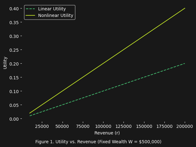
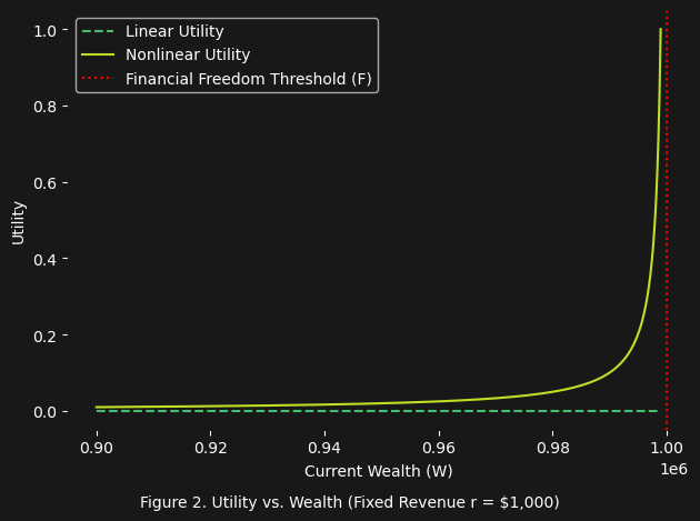
What we see in figure 1 is exactly what we would expect: as the revenue $r$ increases the utility calculated by both the linear and nonlinear functions increases (though the nonlinear is higher simply because it is a smaller denominator: $F = \textdollar1,000,000$ vs. $F - W = \textdollar500,000$). Even the behavior of the two utility functions in figure 1 already gives us a sense that the nonlinear is more meaningful (it considers your existing wealth $W$ into the utility calculation). But figure 2 is where it becomes far more interesting: the utility calculated by the nonlinear function exponentially grows as you approach the financial goal $F$:
\[\lim_{W \to F^{-}} \frac{r}{F - W} = \infty\]This mathematical behavior captures an intuitive truth: the closer you are to achieving your financial goal, the more valuable each dollar of revenue becomes. This creates a sharp, nonlinear incentive to close the gap, and reach that financial goal (i.e. in this case financial freedom).
The Asset Liquidation Problem
In the final section of the article we will focus on a problem taken from the real world, that involves “liquidating” assets in the “best” way possible. These assets can be sold through several distinct methods, each with different prices, effort levels, and capacity constraints. The problem is that each sales method $i$ comes with its own pros/cons:
- Some are fast but come with lower prices.
- Others maximize profit, but require far more time and effort.
- Some involve complex fees, shipping costs, and overhead.
How do we “choose” the best combination of sales methods (i.e. the optimal sales mixed strategy)? We can frame this problem entirely in terms of utility, but now the utility is essentially a “wage” (i.e. profit per time) treating the liquidation process itself as a “job” of sorts.
For each method $i$ we calculate:
\[U_i = \frac{p_i - f_i - s_i}{t_i}\]This tells us the effective wage for using method $i$, where:
- $p_i$ = Price per asset using method $i$
- $f_i$ = Fees per asset (platform fees, transaction costs, etc.)
- $s_i$ = Shipping per asset (if applicable)
- $t_i$ = Time required per asset (total hours to complete sale)
The total utility acquired by selling all the assets via some combination of $n$ sales methods is simply:
\[U_{\text{total}} = \sum_{i=1}^n x_i U_i\]Where $x_i$ is the number of assets sold by method $i$ and $n$ is the total number of methods to consider. But $U_{\text{total}}$ only gives the total utility achieved by selling all the assets, not the average utility per asset (which offers additional insights). So we need to look at the weighted average utility as such:
\[\begin{aligned} N &= \sum_{i=1}^n x_i \\ U_{\text{mean}} &= \frac{U_{\text{total}}}{N} = \frac{1}{N} \sum_{i=1}^n x_i U_i \end{aligned}\]Here $N$ is the total assets to be sold, and $U_{\text{mean}}$ is the weighted average utility. So this problem essentially becomes a maximization problem of the weighted average utility:
\[\max_{x_1, x_2, \dots, x_n} U_{\text{mean}} = \frac{1}{N} \sum_{i=1}^{n} x_i \frac{p_i - f_i - s_i}{t_i}\]Concrete Example
With the theory of how to “liquidate” the assets defined, we are now ready to look at a concrete example. Let’s consider a collection of $N = 100$ assets with $n = 4$ sales methods:
- Method 1: Bulk sale to a local buyer.
- Method 2: Auction through an online platform.
- Method 3: Fixed-price sale through an online marketplace.
- Method 4: Bulk sale to an out-of-state buyer.
And here is the table of data for each method $i$:
| Method | $ p_i $ | $ f_i $ | $ s_i $ | $ t_i $ |
|---|---|---|---|---|
| 1 | 150 | 10 | 0 | 0.5 |
| 2 | 180 | 20 | 5 | 2 |
| 3 | 220 | 15 | 10 | 1.5 |
| 4 | 160 | 10 | 5 | 0.75 |
We can now calculate the utility for each method:
- Method 1: $U_1 = \frac{150 - 10 - 0}{0.5} = 280$
- Method 2: $U_2 = \frac{180 - 20 - 5}{2} = 77.5$
- Method 3: $U_3 = \frac{220 - 15 - 10}{1.5} = 130$
- Method 4: $U_4 = \frac{160 - 10 - 5}{0.75} = 200$
By visual inspection we can easily see that method 1 has the highest utility (i.e. wage) and in the simplest case (where we do not need to consider other constraints like the sales capacity of each method) then the optimal mixed sales strategy is simply:
\[\begin{aligned} \max_{x_1, x_2, x_3, x_4} U_{\text{mean}} &= \frac{1}{N} (x_1 U_1 + 0 U_2 + 0 U_3 + 0 U_4) \\ &= \frac{100 \cdot 280}{100} \\ &= 280 \end{aligned}\]Moral
What utility ultimately does, is allow you to move beyond single terms, like price or revenue, to more complex quantities in order to evaluate which option is “best.” In the “concrete” example above, we are able to balance quantities for revenue/price, costs, and time to arrive at a far superior evaluation of each selling method’s utility (i.e. value). And since the utility we calculate in the aforementioned example is technically a wage, this also allows us to directly compare how “competitive” this “wage” is to a target wage (e.g. the average wage, etc …). Again, thanks to utility we are in a much better position to reason about the overall benefit of not only each sales method compared to each other, but also the resulting “wage” compared to other “jobs.”