Value to Cost Ratio - Higher Level Investment Decisions
Favorable Investment Detection
In the previous article, the following equation was defined and used to calculate the net expected utility:
\[E(n) = (1 - p^n)U - nC\]In the article, a lottery example was used to demonstrate the equation and show objectively which scenario was more advantageous. But this required a much more intensive computation, all to simply show that the second scenario (i.e. the “real” lottery) was completely unfavorable. Is there a better way to determine if some investment is favorable before calculating out the optimal options number $n$?
The Ratio
Consider the following problem: you have a series of investments with known $U$, $C$, and $p$ values, which ones do you choose to further investigate the optimal options number $n$? When this collection of investments is small you can use the original net expected utility equation, but what if you have a non-trivial amount of data? Consider the following collection of investments that require some high-level decision on which are more favorable:
       U        C        p
23628740  8645440 0.000746
   37439    13078 0.464476
19653650   288621 0.966351
 5627542  4508619 0.060871
 8921652  4610030 0.258521
 3589078     1369 0.080797
 7242285   543692 0.920817
 1284134      890 0.415387
 6244378    54235 0.192862
18311837   602570 0.382745
 9287015  7629121 0.281932
17871191  1479129 0.004422
14431905  6896584 0.000053
15094491   306069 0.000551
 1709084    14159 0.528880
 5991814  2618516 0.623773
16564190  4638472 0.441722
23161105 18919224 0.089064
 9198955    71751 0.542063
24563207      271 0.187116
Looking at the above list of investment data can you tell which are more favorable? Should we go through the process of evaluating the net expected utility equation for each pair of $U$, $C$, and $p$ values? No we should not. Instead we should apply the following equation:
\[\frac{(1 - p)U}{C}\]The above equation is a type of risk/reward ratio (in this case reward/risk) and it can be used to get a sense of when a potential investment is favorable (or not).
Return of the Lottery
Now let us apply the previous value/cost ratio to the lottery data from the previous article:
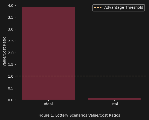
From figure 1 it seems like the threshold for an investment to become favorable is that the value/cost ratio must exceed $1$:
\[\frac{(1 - p)U}{C} > 1\]This would make sense, because this corresponds to the following equation:
\[(1 - p)U = C\]Which is to say that the value and cost terms are equal and when evaluated normally:
\[E(n) = (1 - p)U - C = 0\]So in this case your $E(n) = 0$, i.e. you will not be winning… but at least you will not be losing (i.e. $E(n) < 0$).
Application
Finally we can apply the value/cost ratio to our example investment data and see which are favorable:
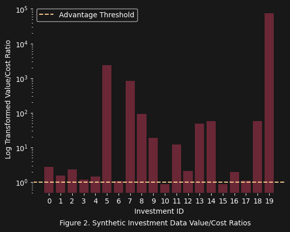
Looking at figure 2 we can easily discern which investments are not favorable, which are barely favorable, which are a little favorable, and finally which investments are reasonably and significantly favorable. But let us now actually apply the original net expected utility and reaffirm that our method works by providing some additional evidence.
Bonus Round
Now let us see how accurate our little value/cost ratio actually is. We will plot the optimal options of the investment data, by grouping them based on their value/cost ratio ($\text{vcr}$) as follows:
not favorable($\text{vcr} < 1$)barely favorable($1 < \text{vcr} < 10$)little favorable($10 < \text{vcr} < 100$)reasonably favorable($100 < \text{vcr} < 5000$)significantly favorable($\text{vcr} > 5000$)
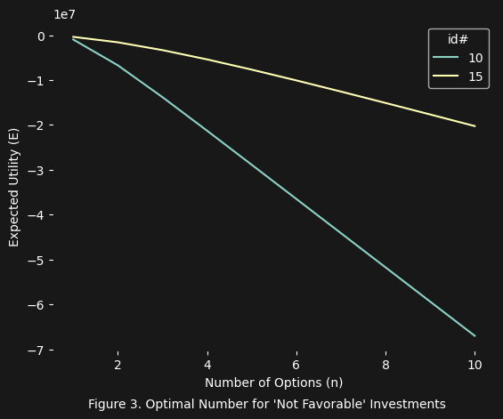
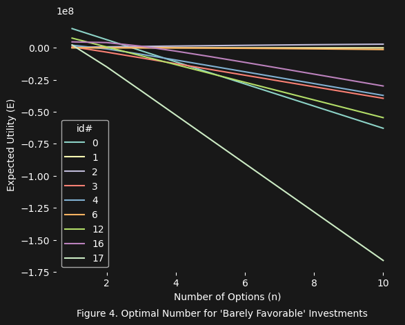
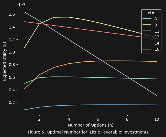
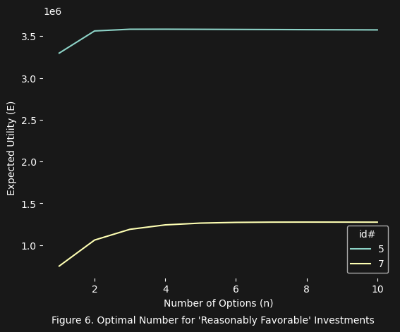
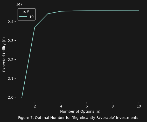
The results are quite interesting (see below data table for investment id lookup). In figure 3 we see basically what we expected (i.e. nothing favorable). In figure 4 there is something interesting happening with the investment ids $1$, $2$, and $6$. And finally in figures 5, 6, and 7 we see what we would expect (several favorable investment options). Of course we also realize from these figures the limits of the value/cost ratio: the ratio alone is not enough to completely filter investment options, unless these options have a $\text{vcr} < 1$ (i.e not favorable). If the $\text{vcr} > 1$, then the particular investment could be favorable. However, the net expected utility equation is still needed to figure out if $E(n)$ decreases as $n$ increases, and if it increases, what the optimal number of options (e.g. the tickets in the lottery) will be.
           U         C         p      vc_ratio
id
0   23628740   8645440  0.000746      2.731049
1      37439     13078  0.464476      1.533070
2   19653650    288621  0.966351      2.291317
3    5627542   4508619  0.060871      1.172197
4    8921652   4610030  0.258521      1.434962
5    3589078      1369  0.080797   2409.855075
6    7242285    543692  0.920817      1.054758
7    1284134       890  0.415387    843.506572
8    6244378     54235  0.192862     92.930296
9   18311837    602570  0.382745     18.758112
10   9287015   7629121  0.281932      0.874112
11  17871191   1479129  0.004422     12.028809
12  14431905   6896584  0.000053      2.092506
13  15094491    306069  0.000551     49.290101
14   1709084     14159  0.528880     56.867280
15   5991814   2618516  0.623773      0.860901
16  16564190   4638472  0.441722      1.993636
17  23161105  18919224  0.089064      1.115177
18   9198955     71751  0.542063     58.710553
19  24563207       271  0.187116  73679.074749
Moral
The power of numbers is not just their objectivity, but also in their ability to obfuscate the truth. As paradoxical as this may sound, what else could be said in regards to the example investment data? It is simply not a simple task to look at columns of numbers and directly determine which will be more favorable in their net expected utility by first impression alone. It is only through a more sharpened application of mathematics (and hence the mind) that we can extract from this infinitude of numbers that mysterious and obscure truth that we desire above all: which investments are favorable?