Housing Competition in One Number - The Price-to-Income Ratio

Introduction

Housing markets are famously complex. Prices are shaped by a tangle of forces: local incomes, job opportunities, migration patterns, zoning restrictions, supply limits, and the influx of outside capital. For most people, this complexity is abstract—until it collides with reality in the form of a sticker shock when house hunting.

Yet, despite all this, there is a surprisingly simple way to gauge the underlying economic competition in any locale: a single ratio. Divide the median home price by the median annual income, and you get a number that tells you, in plain terms, how many years of work it takes for the average person to afford the average home.

This ratio—commonly called the price-to-income multiple—serves as a first-order indicator of housing competition. It captures, in one number, the pressure that buyers face, the scarcity of homes relative to local earning power, and the degree to which external capital or extreme wealth skews the market. In other words, while it cannot explain every detail of a housing market, it reveals how intensely people must compete just to secure a roof over their heads.

In the sections that follow, we’ll define this metric precisely, explain why it works, and explore how it illuminates the economic realities of cities, states, and countries alike.

Defining the Metric

At the core of this analysis is a simple ratio:

\[T = \frac{\text{Median Home Price}}{\text{Median Annual Income}}\]

This quantity—commonly called the price-to-income multiple—measures how many years of income are required for the median household to purchase the median home in a given market.

The interpretation is straightforward. If $T = 5$, then the typical home costs five years of gross income; if $T = 10$, it costs ten. The ratio translates housing from an abstract dollar value into a time-based cost, expressed in units of economic effort. Rather than asking “How expensive is housing?”, it answers a more concrete question: How many years of work does it take to buy a home?

This framing is not just intuitive—it reflects a deeper structure. Housing is a stock (a large, one-time asset), while income is a flow (earned incrementally over time). Dividing the two produces a timescale: the number of years required for income to accumulate into ownership. This makes the metric comparable across regions, allowing fundamentally different markets to be evaluated on a common human scale.

Both components of the ratio are defined using medians, not averages, because income and housing prices are highly skewed distributions. A small number of extremely expensive homes can pull the average price upward, just as a small number of very high earners can distort average income. The median avoids this problem by representing the midpoint: half of homes are cheaper and half are more expensive; half of households earn less and half earn more. As a result, the ratio reflects the economic position of a typical household rather than being distorted by extremes. In unequal markets especially, using averages would systematically understate the true burden of housing.

For completeness, the inverse form can also be defined:

\[r = \frac{\text{Median Annual Income}}{\text{Median Home Price}} = \frac{1}{T}\]

This expresses how much of a house is “earned” per year—a rate rather than a duration. While mathematically equivalent, it is less intuitive. People reason more naturally in terms of time required than fractional accumulation, which is why the price-to-income multiple $T$ serves as the primary formulation. In what follows, we treat $T$ as a fundamental descriptor of a housing market: a compact measure that reduces price, income, and competition to a single, interpretable scale.

Why This Metric Works

At first glance, reducing a housing market to a single ratio may seem like an oversimplification. In reality, the price-to-income multiple works precisely because it captures the outcome of many interacting forces rather than attempting to model them individually.

Housing prices emerge from a competitive bidding process. Buyers—each with different incomes, savings, expectations, and access to credit—compete for a limited supply of homes. The final price reflects the highest bids that can be sustained in that market. As a result, the median home price already encodes a wide range of underlying factors: local wages, job opportunities, migration patterns, supply constraints, and the presence of outside capital.

By dividing price by median income, the metric normalizes this outcome by local earning power. What remains is a measure of how intense that competition is relative to what a typical household can afford. A higher value of $T$ means that buyers must commit more years of income to secure housing, indicating a more competitive and constrained environment. A lower value suggests that housing is more easily attainable relative to local economic conditions.

In this sense, the price-to-income multiple functions as a revealed metric. It does not explain why a market is expensive or affordable; instead, it summarizes the combined effect of all contributing forces in a single observable quantity. Whether high prices are driven by strong job growth, geographic limitations, restrictive zoning, or external investment, the result is the same: an increase in the number of years required to purchase a home.

This is what gives the metric its explanatory power. It compresses a complex system into a single dimension—time—allowing different markets to be compared directly and intuitively. Rather than analyzing dozens of variables, one can look at $T$ and immediately understand the effective level of economic competition for housing in that location.

Real-World Examples Using Housing and Income Data

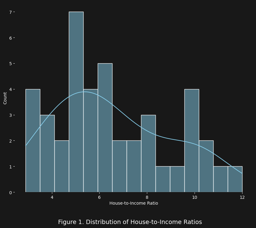
To illustrate the concepts we have explored so far, we examine housing affordability across U.S. cities. Our dataset contains median house prices, median incomes, house-to-income ratios, and recent house price changes.

We begin by examining the overall distribution of house-to-income ratios. This is analogous to observing variance in a simple metric, highlighting how affordability differs across cities.

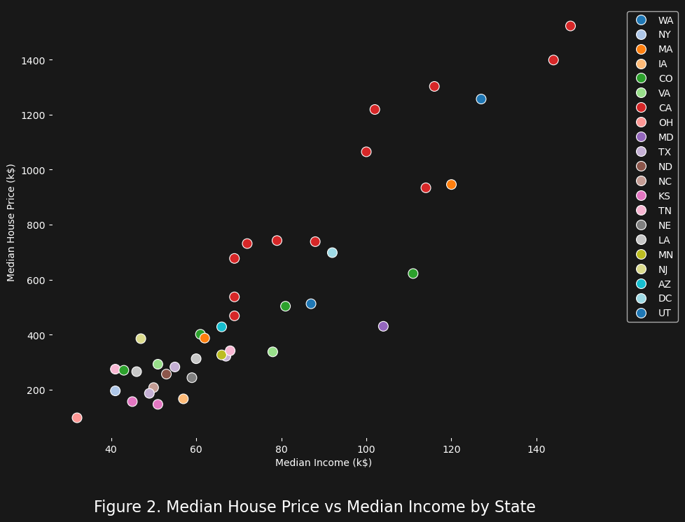
Next, we explore the correlation between median income and median house price, which helps us understand how these two variables interact across different states.

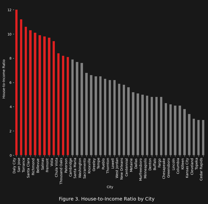
Cities with high house-to-income ratios often represent extreme affordability challenges. Here we highlight cities where the ratio exceeds 8, sorted from highest to lowest.

Finally, we examine the relationship between house price changes and the house-to-income ratio, analogous to monitoring risk and return in a portfolio: higher “risk” (ratio) can sometimes correspond to higher variability (price change).

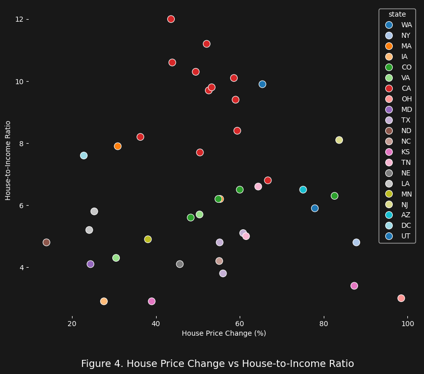
Overall, these examples illustrate variance, extreme values, and covariances in a real dataset. Just as in portfolio theory, attention to outliers and the relationships between variables provides deeper insight into risk and performance.

Conclusion

The price-to-income ratio is a deceptively simple metric, yet as we have seen, it captures the essence of housing affordability pressures across cities. By comparing median home prices to median incomes, we can immediately see where housing markets are most extreme and where residents face the greatest competition just to secure a home.

Our analysis highlighted that certain high-cost cities—such as San Jose, Bellevue, and Fremont—exhibit house-to-income ratios far above the national norm, signaling significant affordability challenges. Meanwhile, many other cities maintain more moderate ratios, reflecting markets where local income levels are more aligned with housing costs.

Visualizing these ratios, with high-ratio cities emphasized, made patterns immediately apparent, showing not just extremes but the relative scale of pressure across different locales. This approach underscores the value of the price-to-income ratio as a first-pass diagnostic tool: it does not capture every nuance of local housing dynamics, but it provides a clear, comparable measure of economic competition for housing.

Ultimately, by combining this metric with careful visualization and data analysis, we gain actionable insight into the intensity of housing pressures, enabling better-informed decisions.