The Meta-Strategy of Eliminating Risk

Introduction

When outcomes are uncertain, simply choosing the option with the highest expected reward is rarely enough. Real-world decisions must account for risk — the volatility, unpredictability, or inconsistency that surrounds expected returns.

But to reason about risk mathematically, we need something more precise. In this article, we treat variance as the formal measurement of risk — the statistical quantity that captures how widely outcomes deviate from their average. When utility functions penalize variance, everything changes:

Any utility function that penalizes variance will naturally converge on an optimal strategy that is not a single option, but a portfolio — a distribution over multiple options.

In other words, risk-aware optimization does not lead to decisions; it leads to distributions. The optimal strategy $\pi^\ast$ is no longer a point on a line, but a vector in strategy space — a blend of options in precise proportions that minimizes uncertainty while maximizing reward.

This shift towards distributional strategies reflects something deeper: a structural rule about how risk-aware systems behave — what we call a meta-strategy. A meta-strategy is not a particular action, but a higher-level design principle. And when risk is penalized — that is, when variance enters the utility function — optimal strategies must become distributed: not single choices, but weighted combinations.

This is not just theoretical elegance. The same pattern appears across domains:

In finance, diversified portfolios reduce variance without sacrificing expected return.
In evolution, organisms hedge reproductive success across environmental niches.
In physics, repeated measurements suppress noise and reveal reliable patterns.
In machine learning, ensembles stabilize predictions by averaging models.

In each case, blending options outperforms betting on just one. It is not merely safer — it is mathematically inevitable.

This inevitability stems from a structural constraint: the variance floor. As we will show, there exists a theoretical minimum level of variance that no single option can ever reach. Only by mixing — by constructing portfolios that exploit negative correlations — can a strategy approach this lower bound.

This limit is not a technicality; it is a proof — the “smoking gun” of the meta-strategy. If variance is penalized, then the optimal response must be a distribution. Not because mixing is preferable, but because it is the only way to reach the minimum. That necessity reveals a deeper truth:

Risk-aware utility functions do not merely encourage diversification — they enforce it.

Mathematical Foundation

The introduction argued that when risk is penalized, optimal decision-making shifts from choosing a single action to distributing weight across several — forming a portfolio. We now make this claim precise.

Let us formalize a setup in which an agent must choose among a finite set of options:

\[\{ x_1, x_2, \dots, x_n \}\]

where each option $x_i$ produces a random return $R_i$. These returns are described by:

Expected return:
\[\mu_i = \mathbb{E}[R_i]\]
Variance:
\[\sigma_i^2 = \mathrm{Var}(R_i) = \mathbb{E}[(R_i - \mu_i)^2]\]
Covariance between any pair of options:
\[\mathrm{Cov}(R_i, R_j) = \mathbb{E}[(R_i - \mu_i)(R_j - \mu_j)]\]

The covariance quantifies how the returns of two options vary together. If two options tend to rise and fall together, their covariance is positive; if they move in opposite directions, it is negative. Zero covariance means the options are uncorrelated.

All pairwise covariances can be organized into a symmetric matrix called the covariance matrix:

\[\Sigma = \begin{bmatrix} \mathrm{Var}(R_1) & \mathrm{Cov}(R_1, R_2) & \cdots & \mathrm{Cov}(R_1, R_n) \\ \mathrm{Cov}(R_2, R_1) & \mathrm{Var}(R_2) & \cdots & \mathrm{Cov}(R_2, R_n) \\ \vdots & \vdots & \ddots & \vdots \\ \mathrm{Cov}(R_n, R_1) & \mathrm{Cov}(R_n, R_2) & \cdots & \mathrm{Var}(R_n) \end{bmatrix}\]

Notice that the diagonal elements of this matrix — $\mathrm{Cov}(R_i, R_i)$ — reduce to the variance of each option:

\[\mathrm{Cov}(R_i, R_i) = \mathbb{E}[(R_i - \mu_i)^2] = \mathrm{Var}(R_i) = \sigma_i^2\]

So, variance is just the special case of covariance where the option is compared with itself. This identity will matter later, when we see that optimal strategies depend on how returns co-vary — not just on how noisy each one is individually.

These quantities — $\mathbb{E}[R_i]$, $\mathrm{Var}(R_i)$, and $\mathrm{Cov}(R_i, R_j)$ — describe how each option behaves, both individually and in relation to others. But understanding the behavior of options is only the first step. To act under uncertainty, the agent must choose a strategy — a rule for selecting among these options. We now distinguish between two types.

Pure vs. Mixed Strategies

A pure strategy selects one option with certainty. For example, choosing only $x_k$ corresponds to the vector:

\[e_k = (0, 0, \dots, 1, \dots, 0)\]

with the 1 in the $k$-th position.

A mixed strategy, by contrast, assigns weights across multiple options. This is expressed as a vector:

\[\pi = (\pi_1, \pi_2, \dots, \pi_n),\]

where:

\[\pi_i \geq 0 \quad \text{for all } i, \quad \text{and} \quad \sum_{i=1}^n \pi_i = 1.\]

This vector defines how the agent distributes effort, probability, or investment across the options. The full set of such vectors forms the strategy simplex, denoted $\Delta^n$ — a geometric space where the corners represent pure strategies and the interior points represent portfolios (i.e. convex combinations of options).

Return and Risk Under Mixed Strategies

If the agent follows a mixed strategy $\pi$, the resulting return is a weighted sum of the individual returns:

\[R_\pi = \sum_{i=1}^n \pi_i R_i\]

The expected return of this strategy is simply the weighted average of the expected returns of each option:

\[\mathbb{E}[R_\pi] = \sum_{i=1}^n \pi_i \mu_i\]

To compute the variance of the return, we must also account for how the individual options co-vary. This includes each option’s own variance and its covariance with every other option. The full expression is:

\[\mathrm{Var}(R_\pi) = \sum_{i=1}^n \sum_{j=1}^n \pi_i \pi_j \mathrm{Cov}(R_i, R_j)\]

This can be written more compactly using matrix notation:

\[\mathrm{Var}(R_\pi) = \pi^\top \Sigma \pi\]

Here, $\pi$ is a column vector of weights:

\[\pi = \begin{bmatrix} \pi_1 \\ \pi_2 \\ \vdots \\ \pi_n \end{bmatrix}, \quad \pi^\top = \begin{bmatrix} \pi_1 & \pi_2 & \cdots & \pi_n \end{bmatrix}\]

and $\Sigma$ is the covariance matrix of the returns:

The matrix form is elegant and efficient, but it is helpful to see how the terms unfold. Expanding the double sum shows that:

The diagonal terms (where $i = j$) contribute the individual variances:
\[\sum_{i=1}^n \pi_i^2 \cdot \mathrm{Var}(R_i)\]
The off-diagonal terms (where $i \ne j$) appear twice due to the symmetry of the covariance matrix:
\[\mathrm{Cov}(R_i, R_j) = \mathrm{Cov}(R_j, R_i)\]

Each pair $(i, j)$ appears both as $\pi_i \pi_j \mathrm{Cov}(R_i, R_j)$ and $\pi_j \pi_i \mathrm{Cov}(R_j, R_i)$, and these terms are equal, so the total becomes:

\[\mathrm{Var}(R_\pi) = \sum_{i=1}^n \pi_i^2 \cdot \sigma_i^2 + 2 \sum_{i<j} \pi_i \pi_j \cdot \mathrm{Cov}(R_i, R_j)\]

This alternate form — sometimes called the bilinear form of portfolio variance — makes the factor of 2 explicit and helps visualize how pairwise relationships influence overall risk.

Growth of Variance and Covariance Terms with Number of Options

An important insight emerges when considering how the number of variance and covariance terms grows as more options are included in the portfolio. The variance terms grow linearly with the number of options $n$, since there is one variance term per option. In contrast, the covariance terms grow quadratically, reflecting the growing number of unique pairs of options whose returns can co-vary.

To illustrate this, consider the following table showing the count of variance and covariance terms as $n$ increases:

Number of Options $n$	Variance Terms	Covariance Terms	Total Terms
1	1	0	1
2	2	2	4
3	3	6	9
4	4	12	16
5	5	20	25
10	10	90	100
20	20	380	400
50	50	2450	2500
100	100	9900	10000

This table reveals a powerful insight:

While variance terms grow only linearly with the number of options, the covariance terms grow quadratically as $\frac{n(n-1)}{2}$, leading to a rapid increase in the potential for interaction effects.
Because covariance terms capture how returns co-vary (positively or negatively), the possibility of reducing overall portfolio variance through diversification grows dramatically as the number of options increases.
In theory, as the number of options becomes very large, well-chosen portfolios can exploit these covariances to annihilate much of the variance, dramatically reducing risk below what any single option offers.

Theoretical Limit of Risk Reduction

As the number of negatively correlated options increases, the potential for variance reduction grows rapidly — not linearly, but quadratically, thanks to the combinatorial explosion of pairwise interactions.

In principle, if enough such anti-correlated options are available, a mixed strategy can reduce total variance to an extremely low level — far below what any single option could achieve. But can variance be driven to zero? Is there a fundamental lower bound?

Let $\Sigma$ be the covariance matrix of $n$ options, and let $\pi$ be a mixed strategy — a weight vector on the n-dimensional probability simplex ($\Delta^n$):

\[\pi \in \Delta^n = \left\{ \pi \in \mathbb{R}^n \mid \sum_{i=1}^n \pi_i = 1,\ \pi_i \geq 0 \right\}\]

As you can see above what $\Delta^n$ represents is the set of all valid mixed strategies where weights are non-negative and sum to 1. Therefore $\pi$ must be a member of the set.

Then the portfolio variance is:

\[\mathrm{Var}(R_\pi) = \pi^\top \Sigma \pi\]

We define the minimum achievable variance across all valid strategies as:

\[\mathrm{Var}_{\min} = \min_{\pi \in \Delta^n} \pi^\top \Sigma \pi\]

This quantity represents the variance floor — the lowest variance achievable by any valid mixed strategy: a weighted average of options where all weights are non-negative and sum to one (i.e. a point in the probability simplex $\Delta^n$).

If $\Sigma$ contains sufficiently many negative covariances — that is, if many pairs of options are anti-correlated — then:

\[\mathrm{Var}_{\min} \ll \min_i \sigma_i^2\]

This inequality means that the optimal mixed strategy produces less variance than even the most stable pure option.

But crucially, no pure strategy can ever achieve this bound. A pure strategy corresponds to a standard basis vector $e_k$, in which:

\[\mathrm{Var}(R_{e_k}) = \sigma_k^2\]

So if:

\[\mathrm{Var}_{\min} < \min_i \mathrm{Var}(R_{e_i}),\]

then only a mixed strategy can achieve it.

Thus, the existence of a theoretical variance minimum that lies below all $\sigma_i^2$ proves the necessity of diversification. The variance-lowering effect of negative covariances is only accessible through a strategy that mixes options. In other words:

The theoretical limit of variance — the “noise floor” — is accessible only through mixing.

This structural asymmetry is the proof that the optimal strategy $\pi^\ast$ for any risk-aware utility function, will be a mixed strategy.

Simulating The Variance Floor

To make the argument concrete, we simulate a decision-making scenario in which an agent chooses among an increasing number of uncertain options. Each option has its own variance, and the options are weakly negatively correlated — meaning their fluctuations tend to partially cancel each other out. We compare two strategies:

Best pure strategy: Select the single option with the lowest individual variance.
Optimal mixed strategy: Choose a portfolio — a weighted combination of options — that minimizes total variance.

As the number of available options $n$ increases, we measure the variance under each strategy. The results are shown in Figure 1 below.

png

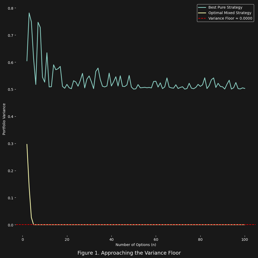
In the figure, the upper curve shows the variance of the best pure strategy — that is, the most stable individual option. As $n$ increases, this value fluctuates slightly but flattens out. In contrast, the lower curve shows the variance achieved by the optimal mixed strategy. It drops rapidly toward a lower bound, approaching what we call the variance floor — the theoretical minimum achievable by any convex combination of the options.

This simulation makes the meta-strategy visible. The more options the system has, the more pairwise covariances it can exploit. And since the number of covariances grows quadratically with $n$, while the number of variances grows only linearly, a mixed strategy gains a dramatic structural advantage. It can coordinate the weights of the portfolio to partially cancel fluctuations — something no single option can do.

This is not a quirk of simulation — it is a mathematical inevitability. As we will now show, the limit of variance reduction is a formal geometric property of the covariance matrix — and its minimum lies strictly inside the strategy simplex, not at its corners.

Conclusion

When utility functions penalize risk (which we measure using variance), a profound shift occurs: optimal strategies cease to be singular choices and instead become structured mixtures. What begins as a pragmatic approach to reducing uncertainty reveals itself as a meta-strategy — a structural rule about the nature of the optimal solution $\pi^\ast$ for risk-aware decision-making.

The existence of a variance floor — a theoretical minimum risk level that no pure strategy can reach — proves this point unequivocally: only mixed strategies can achieve true optimality under uncertainty.

The mathematics leaves no room for compromise:

When risk enters the utility calculation, mixed strategies are not a preference — they are a necessity.